Examine and manipulate stimulus power

This shows how to make stimuli that play at different SNRs and db SPL.

import matplotlib.pyplot as plt
import numpy as np

from expyfun import fetch_data_file
from expyfun.stimuli import read_wav, rms, window_edges

print(__doc__)

Load data

Get 2 seconds of data

data_orig, fs = read_wav(fetch_data_file("audio/dream.wav"))
stop = int(round(fs * 2))
data_orig = window_edges(data_orig[0, :stop], fs)
t = np.arange(data_orig.size) / float(fs)

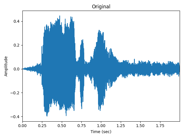
# look at the waveform
fig, ax = plt.subplots()
ax.plot(t, data_orig)
ax.set(xlabel="Time (sec)", ylabel="Amplitude", title="Original", xlim=t[[0, -1]])
fig.tight_layout()

2024-07-22 22:15:11,346 - INFO    - Read WAV file with 1 channel and 414951 samples (format int16)

Normalize it

expyfun.ExperimentController by default has stim_rms=0.01. This means that audio samples normalized to an RMS (root-mean-square) value of 0.01 will play out at whatever stim_db value you supply (during class initialization) when the experiment is deployed on properly calibrated hardware, typically in an experimental booth. So let’s normalize our clip:

print(rms(data_orig))
target = data_orig / rms(data_orig)
target *= 0.01
# do manual calculation same as ``rms``, result should be 0.01
# (to numerical precision)
print(np.sqrt(np.mean(target**2)))

0.08416927712570585
0.009999999999999998

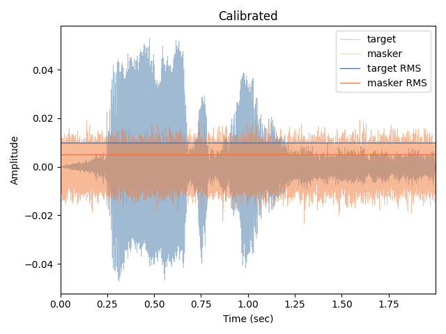
One important thing to note about this stimulus is that its long-term RMS (over the entire 2 seconds) is now 0.01. There will be quiet parts where the RMS is effectively lower (close to zero) and louder parts where it’s bigger.

Add some noise

Now let’s add some masker noise, say 6 dB down (6 dB target-to-masker ratio; TMR) from that of the target.

Note

White noise is used here just as an example. If you want continuous white background noise in your experiment, consider using ec.start_noise() and/or ec.set_noise_db() which will automatically keep background noise continuously playing during your experiment.

# Good idea to use a seed for reproducibility!
ratio_dB = -6.0  # dB
rng = np.random.RandomState(0)
masker = rng.randn(len(target))
masker /= rms(masker)  # now has unit RMS
masker *= 0.01  # now has RMS=0.01, same as target
ratio_amplitude = 10 ** (ratio_dB / 20.0)  # conversion from dB to amplitude
masker *= ratio_amplitude

Looking at the overlaid traces, you can see that the resulting SNR varies as a function of time.

colors = ["#4477AA", "#EE7733"]
fig, ax = plt.subplots()
ax.plot(t, target, label="target", alpha=0.5, color=colors[0], lw=0.5)
ax.plot(t, masker, label="masker", alpha=0.5, color=colors[1], lw=0.5)
ax.axhline(0.01, label="target RMS", color=colors[0], lw=1)
ax.axhline(0.01 * ratio_amplitude, label="masker RMS", color=colors[1], lw=1)
ax.set(xlabel="Time (sec)", ylabel="Amplitude", title="Calibrated", xlim=t[[0, -1]])
ax.legend()
fig.tight_layout()

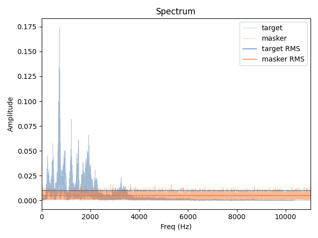
Examine spectra

We can also look at the spectra of these stimuli to get a sense of how the SNR varies as a function of frequency.

from scipy.fft import rfft, rfftfreq  # noqa

f = rfftfreq(len(target), 1.0 / fs)
T = np.abs(rfft(target)) / np.sqrt(len(target))  # normalize the FFT properly
M = np.abs(rfft(masker)) / np.sqrt(len(target))
fig, ax = plt.subplots()
ax.plot(f, T, label="target", alpha=0.5, color=colors[0], lw=0.5)
ax.plot(f, M, label="masker", alpha=0.5, color=colors[1], lw=0.5)
T_rms = rms(T)
M_rms = rms(M)
print("Parseval's theorem: target RMS still %s" % (T_rms,))
print("dB TMR is still %s" % (20 * np.log10(T_rms / M_rms),))
ax.axhline(T_rms, label="target RMS", color=colors[0], lw=1)
ax.axhline(M_rms, label="masker RMS", color=colors[1], lw=1)
ax.set(xlabel="Freq (Hz)", ylabel="Amplitude", title="Spectrum", xlim=f[[0, -1]])
ax.legend()
fig.tight_layout()

Parseval's theorem: target RMS still 0.009999773251761586
dB TMR is still 5.99988977063175